Labeled Latent Dirichlet Allocation (LLDA)

引言

建議先看過 Latent Dirichlet Allocation (LDA) 後再閱讀本文。

現今有不少文本帶有標籤 (label)，例如新聞文章會有「交通」與「政治」等各式標籤，並且這些標籤彼此並沒有明顯的子集關係。傳統 LDA 是一種非監督式學習，有時會分類出難以標記的主題，並且也無從驗證其真實應用性，而 Labeled Latent Dirichlet Allocation (LLDA) 提出直接從 LDA 的主題直接學習與標籤的關係，以此建構出以文本預測類別的監督式學習。

定義

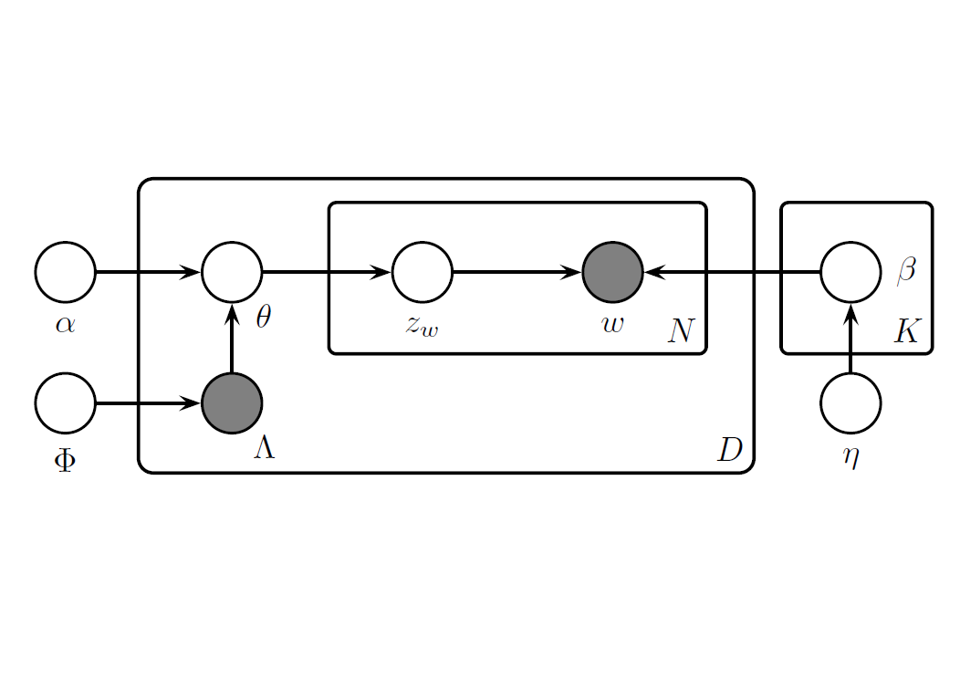
給定一文件 $d$，其包含字詞表 $w^{(d)} = (\contia{w}{N_d})$ 與 0, 1 紀錄的標籤 $\Lambda^{(d)} = (\contia{l}{K})$，其中 $w_i \in \{ \conti{V} \}$ 且 $l_k \in \{ 0, 1 \}$，$N_d$ 表示文件長度，$V$ 表示總單字量，$K$ 表示標籤總數。

並包含 2 個參數，$\eta \in \bb R^V$ 表示單字的 prior、$\alpha \in \bb R^K$ 表示主題的 prior

文件生成

LDA 假設文本生成服從以下分布

1. 生成各主題下的單字分布 $\beta_k \sim \text{Dir} (\eta)$ 對 $k = \conti{K}$
2. 生成各文件下的主題分布 $\theta^{(d)} \sim \text{Dir} (\alpha)$ 對 $d = \conti{D}$
3. 生成文件下的單字
   1. 選定每個位置的主題 $z_i \sim \text{Mult} ( \theta^{(d)} )$ 對 $i = \conti{N_d}$
   2. 選定每個位置的單字 $w_i \sim \text{Mult} ( \beta_{z_i} )$ 對 $i = \conti{N_d}$

相較於 LDA 假設文件是所有主題的 Dirichlet 分布，LLDA 假設文件是其包含標籤的 Dirichlet 分布，因此對修改了第 2 步的主題分布

第 2 步中，LLDA 假設文件生成時會依照 Bernoulli 分布決定是否包含某標籤，以 $\Phi_k$ 的機率擁有第 $k$ 種標籤，即 $\Lambda_{k}^{(d)} \sim \ber (\Phi_k)$，以 $\lambda^{(d)} = \{ k : \Lambda_{k}^{(d)} = 1 \}$ 紀錄擁有的標籤，以 $M_d = |\lambda^{(d)}|$ 表示文件擁有的標籤量，並以 $L^{(d)} \in \bb R^{M_d \times K}$ 限縮主題 $\alpha$ 的採樣範圍，即

並以 $\alpha^{(d)}$ 表示被限縮後的空間

LLDA 假設文本生成服從以下分布

1. 生成各主題下的單字分布 $\beta_k \sim \text{Dir} (\eta)$ 對 $k = \conti{K}$
2. 生成各文件下的主題分布 $\theta^{(d)}$ 對 $d = \conti{D}$
   1. 生成主題 $\Lambda_k^{(d)} \sim \ber (\Phi_k)$ 對 $k = \conti{K}$
   2. 獲取限縮後的主題分布 $\alpha^{(d)} = L^{(d)} \alpha$
   3. 生成主題分布 $\theta^{(d)} \sim \text{Dir} (\alpha^{(d)})$
3. 生成文件下的單字
   1. 選定每個位置的主題 $z_i \sim \text{Mult} ( \theta^{(d)} )$ 對 $i = \conti{N_d}$
   2. 選定每個位置的單字 $w_i \sim \text{Mult} ( \beta_{z_i} )$ 對 $i = \conti{N_d}$

範例

例如 $K = 4$ 表示有 4 個主題，若第 $d$ 份文件包含 2 與 3 號主題，則 $\Lambda^{(d)} = (0, 1, 1, 0)$、$\lambda^{(d)} = \{ 2, 3 \}$ 和

使得

即 $d$ 包含幾號標籤，則 $\alpha^{(d)}$ 就有幾號標籤，文件的主題分布會僅會在 $\alpha_2$ 與 $\alpha_3$ 中採樣，例如 $(\alpha_2, \alpha_3) = (0.3, 0.7)$；而非在所有的 $4$ 主題中採樣

參數估計

對參數估計，會透過 collapsed Gibbs sampling 進行，迭代方式如下

會發現此訓練方式與原始 LDA 的方式相同，唯一的差別在於限制限制在文本帶有的標籤中，即 $j \in \lambda^{(d)}$。

當 $\beta$ 從訓練集訓練完後，可以對新文件進行推論，以 Gibbs sampling 決定每個單字的主題。經過觀察文中各單字所分配的主題分布，以此決定決定該文件的主題分布 $\theta$

LLDA 除了 $\beta$ 的估計方法與 LDA 不同，其餘如新文件的主題推論、關鍵字視覺化等都與 LDA 的方法相同

Naive Bayes 的關聯

考慮每個文本僅有單一標籤時，LLDA 可以被視為是 Naive Bayes Learning 的延伸，LLDA 得先抽取各個位置單字的主題後再抽取用字，但在單一標籤抽籤時能抽出的也只有一種可能，即 $z_i = \lambda_1^{(d)}$ 對任意 $i \in \{ \conti{V} \}$，使得文件的每個單字能直接對應到 $\beta_{\lambda_1^{(d)}, w_i}$，因而各文件在 LLDA 下的機率與 Multinomial Naive Bayes classifier 下的機率相同

但 LLDA 與 Naive Bayes Learning 的關係僅至單一標籤，若文件含有多個標籤，Naive Bayes 中每個單字會對文本所包含的標籤貢獻均加 1；而 LLDA 會對觀察到的單字生成標籤，使得單字僅對單一標籤貢獻加 1

Python 套件 tomotopy

Topic Modeling Tool in Python (tomotopy) 是 python 中用 Gibbs sampling 實作的套件

20 Newsgroups

以熱門的 20 Newsgroups 資料集作為範例，以郵件形式呈現的 20 種新聞主題，在 sklearn.datasets 可以直接使用

import numpy as np
import pandas as pd
from sklearn.datasets import fetch_20newsgroups

# get train data
fetch = fetch_20newsgroups(subset="train", remove=('footers', "quotes"))
train = pd.DataFrame({'label': fetch.target, 'content': fetch.data})
train['label'] = train['label'].map(lambda x: fetch.target_names[x])

# get test data
fetch = fetch_20newsgroups(subset="test", remove=('footers', "quotes"))
test = pd.DataFrame({'label': fetch.target, 'content': fetch.data})
test['label'] = test['label'].map(lambda x: fetch.target_names[x])

print(train.head)
pythonCopy

輸出 train set

                          label                                            content
0                     rec.autos  From: lerxst@wam.umd.edu (where's my thing)\nS...
1         comp.sys.mac.hardware  From: guykuo@carson.u.washington.edu (Guy Kuo)...
2         comp.sys.mac.hardware  From: twillis@ec.ecn.purdue.edu (Thomas E Will...
3                 comp.graphics  From: jgreen@amber (Joe Green)\nSubject: Re: W...
4                     sci.space  From: jcm@head-cfa.harvard.edu (Jonathan McDow...
                        ...                                                ...
11309                   sci.med  From: jim.zisfein@factory.com (Jim Zisfein) \n...
11310     comp.sys.mac.hardware  From: ebodin@pearl.tufts.edu\nSubject: Screen ...
11311  comp.sys.ibm.pc.hardware  From: westes@netcom.com (Will Estes)\nSubject:...
11312             comp.graphics  From: steve@hcrlgw (Steven Collins)\nSubject: ...
11313           rec.motorcycles  From: gunning@cco.caltech.edu (Kevin J. Gunnin...

[11314 rows x 2 columns]>
 Copy

EDA

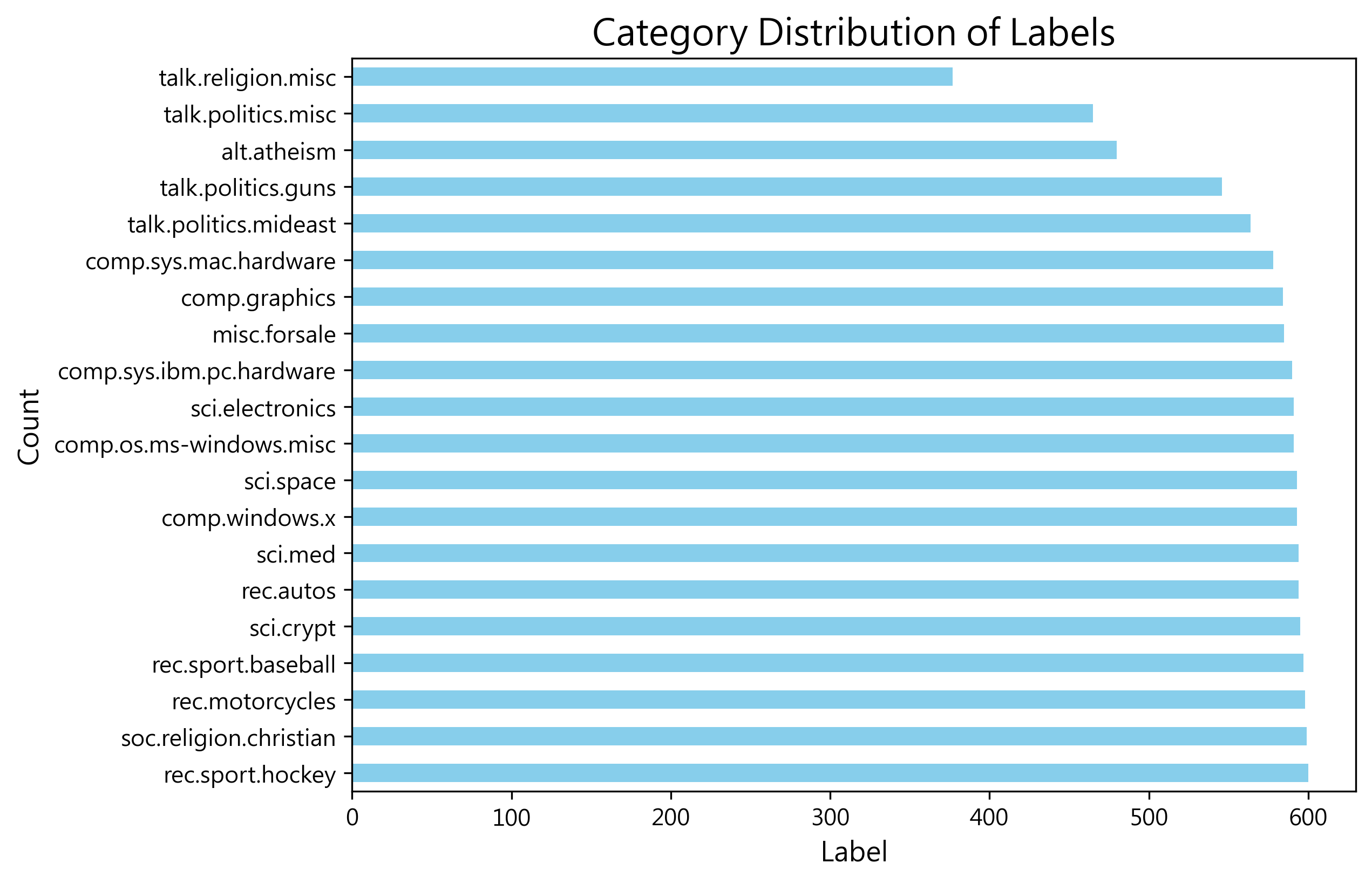
查看其類別分類，20 類別分布頗為平均

#%% EDA
import matplotlib.pyplot as plt

label_counts = train.label.value_counts()

# figure size
plt.figure(figsize=(8, 6)) 
# bar chart
label_counts.plot(kind='barh', color='skyblue') 

# add text
plt.title('Category Distribution of Labels', fontsize=16)
plt.xlabel('Label', fontsize=12)
plt.ylabel('Count', fontsize=12)

# show figure
plt.show()
pythonCopy

文本預處理

對文本預處理，詳見 預處理

#%% preprocess content
import re
import nltk
from nltk.corpus import stopwords
from nltk.stem import WordNetLemmatizer
from nltk.tokenize import word_tokenize

# Make sure downloaded the nltk resources
nltk.download('punkt')
nltk.download('punkt_tab')
nltk.download('stopwords')
nltk.download('wordnet')

stop_words = set(stopwords.words('english'))
lemmatizer = WordNetLemmatizer()

def preprocess(text):
    # to lower
    text = str(text).lower()
    
    # remove symbol
    text = re.sub(r'[^a-zA-Z\s]', ' ', text)
    
    # tokenize
    tokens = word_tokenize(text)
    
    # stop word
    tokens = [word for word in tokens if word not in stop_words]
    
    # lemmatization
    tokens = [lemmatizer.lemmatize(word) for word in tokens]
    
    return tokens

# processed text
train['processed_content'] = train['content'].apply(preprocess)
test['processed_content'] = test['content'].apply(preprocess)
pythonCopy

並將文本轉換成 tomotopy 支援的 Corpus 格式

#%% Content to corpus 
import tomotopy as tp
from tomotopy.utils import Corpus

# creat a corpus
train_corpus = Corpus()
test_corpus = Corpus()

# add content and label
for index, row in train.iterrows():
    train_corpus.add_doc(words=row['processed_content'], labels=[row['label']])
    
for index, row in test.iterrows():
    test_corpus.add_doc(words=row['processed_content']) 
pythonCopy

Training

llda_model.train 中的第一個參數表示迭帶次數，這邊以 100 次做為示範

#%% train LLDA
# creat a llda model
llda_model = tp.PLDAModel(tw = tp.TermWeight.IDF) # use tf-idf

# put in the corpus
llda_model.add_corpus(train_corpus)

# training modeling, set the number of train
llda_model.train(100, show_progress = True)
pythonCopy

查看訓練後的結果

#%% LLDA diagnosis
llda_model.summary()

# print the first 20 item in topic
for i in range(llda_model.k):
    print(llda_model.topic_label_dict[i])
    for j in llda_model.get_topic_words(i, top_n = 20):
        print(j)
    print()
pythonCopy

<Basic Info>
| PLDAModel (current version: 0.13.0)
| 11314 docs, 1415731 words
| Total Vocabs: 69821, Used Vocabs: 69821
| Entropy of words: 8.66584
| Entropy of term-weighted words: 9.56597
| Removed Vocabs: <NA>
| Label of docs and its distribution
|  rec.autos: 594
|  comp.sys.mac.hardware: 578
|  comp.graphics: 584
|  sci.space: 593
|  talk.politics.guns: 546
|  sci.med: 594
|  comp.sys.ibm.pc.hardware: 590
|  comp.os.ms-windows.misc: 591
|  rec.motorcycles: 598
|  talk.religion.misc: 377
|  misc.forsale: 585
|  alt.atheism: 480
|  sci.electronics: 591
|  comp.windows.x: 593
|  rec.sport.hockey: 600
|  rec.sport.baseball: 597
|  soc.religion.christian: 599
|  talk.politics.mideast: 564
|  talk.politics.misc: 465
|  sci.crypt: 595
|
<Training Info>
| Iterations: 100, Burn-in steps: 0
| Optimization Interval: 10
| Log-likelihood per word: -8.50162
|
<Initial Parameters>
| tw: TermWeight.IDF
| min_cf: 0 (minimum collection frequency of words)
| min_df: 0 (minimum document frequency of words)
| rm_top: 0 (the number of top words to be removed)
| latent_topics: 0 (the number of latent topics, which are shared to all documents, between 1 ~ 32767)
| topics_per_label: 1 (the number of topics per label between 1 ~ 32767)
| alpha: [0.1] (hyperparameter of Dirichlet distribution for document-topic, given as a single `float` in case of symmetric prior and as a list with length `k` of `float` in case of asymmetric prior.)
| eta: 0.01 (hyperparameter of Dirichlet distribution for topic-word)
| seed: 1667601163 (random seed)
| trained in version 0.13.0
|
<Parameters>
| alpha (Dirichlet prior on the per-document topic distributions)
|  [0.00356926 0.00349817 0.0035254  0.00356774 0.00336278 0.00357206
|   0.00355272 0.00355636 0.00358601 0.00337346 0.00353067 0.0024621
|   0.00355752 0.00356748 0.00359557 0.00358171 0.00359369 0.00344383
|   0.00214761 0.00357747]
| eta (Dirichlet prior on the per-topic word distribution)
|  0.01
|
<Topics>
| Label rec.autos-0 (#0) (48607) : car engine auto oil tire
| Label comp.sys.mac.hardware-0 (#1) (46686) : mac apple drive scsi mb
| Label comp.graphics-0 (#2) (68023) : image graphic jpeg file format
| Label sci.space-0 (#3) (84062) : space nasa launch satellite orbit
| Label talk.politics.guns-0 (#4) (73545) : gun firearm weapon handgun law
| Label sci.med-0 (#5) (79521) : pitt patient geb gordon msg
| Label comp.sys.ibm.pc.hardware-0 (#6) (55565) : drive scsi controller ide card
| Label comp.os.ms-windows.misc-0 (#7) (100710) : ax w q z f
| Label rec.motorcycles-0 (#8) (46490) : bike dod motorcycle ride helmet
| Label talk.religion.misc-0 (#9) (49120) : god jesus christian bible morality
| Label misc.forsale-0 (#10) (48962) : sale offer do shipping price
| Label alt.atheism-0 (#11) (56268) : atheist god atheism religion argument
| Label sci.electronics-0 (#12) (53925) : wire circuit wiring outlet ground
| Label comp.windows.x-0 (#13) (103583) : x entry widget file window
| Label rec.sport.hockey-0 (#14) (73269) : team game hockey pt nhl
| Label rec.sport.baseball-0 (#15) (48345) : game player team baseball year
| Label soc.religion.christian-0 (#16) (83437) : god jesus christian church christ
| Label talk.politics.mideast-0 (#17) (111316) : armenian turkish israel israeli jew
| Label talk.politics.misc-0 (#18) (77080) : stephanopoulos q president mr tax
| Label sci.crypt-0 (#19) (107217) : key db encryption clipper chip
 Copy

Inference

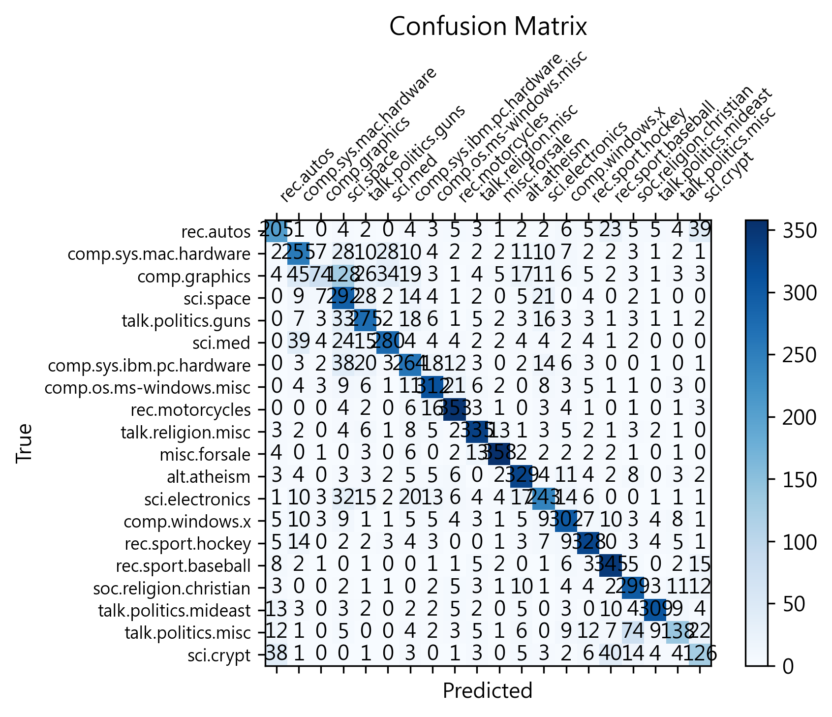
查看其對 test set 表現，用 llda_model.infer 對新文件推論其主題分布

#%% infer new corpus
topic_dist, ll = llda_model.infer(test_corpus)
pythonCopy

用 sklearn.metrics 的 accuracy_score 查看預測精確度

#%% diagnosis LLDA with test accuracy
from sklearn.metrics import accuracy_score

# the real label
real_labels = test.label.tolist()
# the prediction label
predicted_labels = []

for doc in topic_dist:
    # print(list(doc)) # print a list of words within the document
    # print(doc.get_topics()) # print a list of words within the document
    topics = doc.get_topics()
    
    # get topics
    predicted_topic = topics[0][0]
    
    # get topics label
    predicted_label = llda_model.topic_label_dict[predicted_topic]
    predicted_labels.append(predicted_label)
    
print("test acc:", accuracy_score(real_labels, predicted_labels))
pythonCopy

test acc: 0.7198619224641529
 Copy

用 sklearn.metrics 的 confusion_matrix 查看其混淆矩陣

#%% diagnosis LLDA with test accuracy confusion matrix
from sklearn.metrics import confusion_matrix

cm = confusion_matrix(real_labels, predicted_labels)

# 設定中文字體
plt.rc('font', family='Microsoft JhengHei')

# 設置圖形大小為 1920x1080
plt.figure(figsize=(6.4, 6.4), dpi = 300)

# 繪製混淆矩陣
fig, ax = plt.subplots()
cax = ax.matshow(cm, cmap='Blues')

# 設置標籤
plt.title('Confusion Matrix')
ax.set_xlabel('Predicted')
ax.set_ylabel('True')

num_classes = cm.shape[0]  # 類別數量
ax.set_xticks(np.arange(num_classes)) # 設定 x 數值
ax.set_yticks(np.arange(num_classes)) # 設定 y 數值
ax.set_xticklabels(llda_model.topic_label_dict) # 設定 x 圖標
ax.set_yticklabels(llda_model.topic_label_dict) # 設定 y 圖標

# 設置字體大小
plt.xticks(fontsize=8)  # x 軸刻度標籤字體大小
plt.yticks(fontsize=8)  # y 軸刻度標籤字體大小

# 設置 x 軸刻度標籤的旋轉角度
plt.xticks(rotation=45, ha='left')

# 在每個方格中添加數值
for (i, j), value in np.ndenumerate(cm):
    ax.text(j, i, value, ha='center', va='center', color='black')

# 添加顏色條
plt.colorbar(cax)

# plt.tight_layout()

plt.savefig('my_plot.png', dpi = 300, bbox_inches='tight')

plt.show()
pythonCopy

參考資料

1. Ramage, D., Hall, D., Nallapati, R., and Manning, C. D. (2009), “Labeled LDA: a supervised topic model for credit attribution in multi-labeled corpora,” in Proceedings of the 2009 Conference on Empirical Methods in Natural Language Processing Volume 1 - EMNLP ’09, Singapore: Association for Computational Linguistics, p. 248. https://doi.org/10.3115/1699510.1699543.