
垃圾郵件分類機器學習
引言
封面是 Bing 繪製的「垃圾郵件分類器」。
應用 文字探勘 技術,建立出能分類出正常與垃圾郵件的分類器,資料來自 Spam Text Message Classification,資料大小是 5572 x 2,目標是根據 Message 內容預測 Category 是 ham or spam。
| Category | Message |
|---|---|
| ham | Go until jurong point, crazy.. Available only … |
| ham | Ok lar… Joking wif u oni… |
| spam | Free entry in 2 a wkly comp to win FA Cup fina… |
| ham | U dun say so early hor… U c already then say… |
| ham | Nah I don’t think he goes to usf, he lives aro… |
站在巨人肩膀上
參考 其他人的成果,最高的 test accuracy 約在 96% 左右,前幾名的做法大致是
- EDA
- 移除重複值
- Message 預處理:
- 全文字轉小寫
- 移除標點符號
- 移除數字內容
- 移除停用字 (stop words, e.g. I, me, the 等字)
- 字幹提取 (Stemming, e.g. running 和 ran 還原成 run)
- 向量化 (Vectorization)
- TF-IDF (term frequency–inverse document frequency)
- Modeling
- Random forest
- Multinomial Naive Bayes
反省
一開始的 train accuracy 約是 80%,隨著對資料的 EDA 增加,精確度慢慢爬升 90%、95%、98%,到最後的 100%!最終的 test accuracy 約是 99%,這次經歷學到
- 別人的東西參考就好,不一定是最好
- EDA 超級重要,fearture engineering 做的好能大幅度提升模型表現
其他人的 EDA 有計算字元 (character)、單字 (word) 和句子 (sentence) 數量,並發現語句長度與是否為垃圾郵件的關係,但建模卻沒有用上,而大家常用的步驟也不一定是最好的步驟,因此提出以下問題
- 字元、字數和語句數量是種 fearture 嗎?
- 停用字真的該停用嗎?i、me、we 這些字真的不能用嗎?
- 標點符號真的沒用嗎?
Explore Data Analysis
這筆資料含有約 7.4% 的重複值 (例如第 8, 104, 155 筆資料),移除後資料大小為 5157。
預測目標是不平衡的 ham 87.6%,而 spam 12.4%。其中字元 (character)、單字 (word) 與句子 (sentence) 的密度圖,能看出越長的語句越有可能是垃圾郵件


相關性矩陣也顯示出相同的結論

Pre-processing
將資料分成 70% train,30% test,接續的預處理與建模都只用到 train 出現的字,而非所有出現過的字。
跟著其他人的預處理步驟,將 stop word 移除後觀察,在正常郵件中 u 出現在 14% 篇訊息中, go 出現在 8% 篇訊息中,依此類推。

在垃圾郵件中,愛用字是 call、now、free 等字眼

用正常郵件的文字出現率減去垃圾郵件的文字出現率,能看出兩種郵件用字的差距範圍落在 5% 至 -37%

Stop Word
停用字真的該停用嗎?i、me、we 這些字真的不能用嗎?現在不移除停用字,把所有文字考慮進去,並用紅色表示 stopword。
in、if 等字是保留字元,會導致後續建模問題,改用 num_in 和 num_if 取代。

兩種郵件用字的差距範圍落在 26% 至 -37%
標點符號
標點符號真的不考慮嗎?現在考慮 £ (英鎊符號) 與 !,並用 num_pound 和 num_exclam,用紅色表示:

所有標點符號 (num_punct) 和 . (句號, num_period) 在垃圾郵件的出現率也比正常郵件高了約 10%,雖然比不上前面幾名,但也是能提供預測效力的特徵。
Modeling
這次建模選用 Multinomial Naive Bayes,其運算量少,計算速度極高。
常用的方式不考慮字元數量、移除 stop word、移除標點符號,test accuracy 約在 96% 左右,後續每多做一點 feature 就能多 1% 的精確度。
最終結果 Train Accuracy: 100%、Test Accuracy: 98.9%
Test Confusion Matrix:
| Reference | |||
|---|---|---|---|
| ham | spam | ||
Prediction | ham | 1342 | 12 |
| spam | 5 | 187 | |
Code
library(dplyr) # %>%

library(DataExplorer) # EDA
library(ggplot2) # plot

library(stringr) # text process
library(tm) # text mining
library(SnowballC) # stemDocument

library(caret) # train
library(naivebayes) # Naive Bayes Classifier
library(ROCR) # ROC and AUC
EDA
# read data
data = read.csv("spam.csv", fileEncoding = "UTF-8") %>%
  mutate(Category = factor(Category))
data$Category_num = ifelse(data$Category == "ham", 0, 1)
# calculate the number of character, word and sentence
data$num_character = nchar(data$Message)
data$num_word = lapply(data$Message, function(text){
  length(unlist(strsplit(text, "\\s+")))
  }) %>% unlist()
data$num_sentence = lapply(data$Message, function(text){
  length(unlist(strsplit(text, "[.!?]+")))
  }) %>% unlist()
# check missing value and duplicated
data$Message %>% is.na() %>% sum()
data$Message %>% duplicated() %>% sum()

# remove duplicated
data = data[! duplicated(data$Message), ]
# proportion of ham and spam
data$Category %>% table() %>% prop.table()
# correlation plot
plot_correlation(
  data[, c("Category_num", "num_character", "num_word", "num_sentence")],
  theme_config = list(axis.text.x = element_text(angle = 45))
)
plot_densities = function(indexs, bw = 1){
  for(index in indexs){
    density_ham = data[data$Category == "ham", index] %>% density(from = 0, bw = bw)
    density_ham_x = density_ham$x %>% range()
    density_ham_y = density_ham$y %>% range()

    density_spam = data[data$Category == "spam", index] %>% density(from = 0, bw = bw)
    density_spam_x = density_spam$x %>% range()
    density_spam_y = density_spam$y %>% range()

    plot(density_ham,
         xlim = c(min(density_ham_x[1], density_spam_x[1]),
                  max(density_ham_x[2], density_spam_x[2])),
         ylim = c(min(density_ham_y[1], density_spam_y[1]),
                  max(density_ham_y[2], density_spam_y[2])),
         main = paste("Density plot of", index), xlab = index,
         col = "green", )
    lines(density_spam, col = "red")
    legend("topright", legend = c("spam", "ham"), pch = 16, col = c("red", "green"))
  }
}

c("num_character", "num_word", "num_sentence") %>% plot_densities()
Pre-processing
# sampling
set.seed(0)
train_index = createDataPartition(data$Category, p = 0.7, list = F)
train = data[train_index, ]
test = data[-train_index, ]
# transform message to corpus
corpus = Corpus(VectorSource(train$Message))

# processing
corpus = corpus %>%
  tm_map(content_transformer(tolower)) %>% # text becomes lowercase
  tm_map(removePunctuation) %>% # remove punctuation
  tm_map(removeNumbers) %>% # remove numbers
  tm_map(stripWhitespace) %>% # strip white space
  tm_map(stemDocument) # stemming
  # tm_map(removeWords, stopwords("english")) # remove stop words

# £ to pound_sign, in to intransform, the following word are reserve word in modeling
custom_replace = function(x) {
  x = gsub("£", " num_pound ", x, fixed = TRUE)
  x = gsub("\\bin\\b", "num_in", x, ignore.case = TRUE)
  x = gsub("\\bfor\\b", "num_for", x, ignore.case = TRUE)
  return(x)
}

corpus = corpus %>% tm_map(content_transformer(custom_replace))
Document Term Matrix
# number of punctuation
punctuation = data.frame(num_punct = str_count(train$Message, "[[:punct:]]"),
                         num_exclam = str_count(train$Message, "!"),
                         num_period = str_count(train$Message, "\\.")) %>%
  data.matrix()
# document to term matrix
dtm = DocumentTermMatrix(corpus, control = list(wordLengths = c(1, Inf)))
dtm_matrix = as.matrix(dtm)
dtm_matrix = punctuation %>% cbind(dtm_matrix)
new_train = cbind(train, dtm_matrix)
# check the different between ham and spam
non_zero_ham = apply(t(dtm_matrix[which(train$Category == "ham"), ]), 1, function(row) sum(row != 0)) / sum(train$Category == "ham")
non_zero_spam = apply(t(dtm_matrix[which(train$Category == "spam"), ]), 1, function(row) sum(row != 0)) / sum(train$Category == "spam")

diff = (non_zero_ham - non_zero_spam) %>% sort(decreasing = T)

head(diff, 10)
tail(diff, 10)
# 處理 test data
test_corpus = Corpus(VectorSource(test$Message))

# 預處理
test_corpus = test_corpus %>%
  tm_map(content_transformer(tolower)) %>% # 小寫字母
  tm_map(removePunctuation) %>% # 移除標點符號
  tm_map(removeNumbers) %>% # 移除數字
  tm_map(stripWhitespace) %>% # 移除空白
  tm_map(stemDocument) %>% # 詞幹提取 stemming
  tm_map(content_transformer(custom_replace))
  # tm_map(removeWords, stopwords("english")) # 移除無意義字
# number of punctuation
test_punctuation = data.frame(num_punct = str_count(test$Message, "[[:punct:]]"),
                              num_exclam = str_count(test$Message, "!"),
                              num_period = str_count(test$Message, "\\.")) %>%
  data.matrix()
# document to term matrix
test_dtm = DocumentTermMatrix(test_corpus, control = list(dictionary = Terms(dtm)))
test_dtm_matrix = as.matrix(test_dtm)
test_dtm_matrix = test_punctuation %>% cbind(test_dtm_matrix)
new_test = cbind(test, test_dtm_matrix)
modeling
# over sample
oversample = upSample(x = new_train %>% select(-"Category"),
                      y = new_train$Category,
                      yname = "Category")
diff_term = 30

diff_name = diff %>% names() %>% head(diff_term)
diff_name = diff %>% names() %>% tail(diff_term) %>% c(diff_name)

forumla = paste("Category ~ num_character + num_word + num_sentence + ", paste(diff_name, collapse = " + ")) %>%
  as.formula()
# train control
train_control = trainControl(method = "cv", number = 10)
Random Forest
# random forest
set.seed(0)
rf = train(forumla,
           data = new_train,
           trControl = train_control,
           method = "rf")
# train performance
predictions = predict(rf, newdata = new_train)
confusionMatrix(new_train$Category, predictions)
# ROC/AUC
predicted_prob = predict(rf, newdata = new_train, type = "prob")
prediction = prediction(predicted_prob[, 2], new_train$Category)
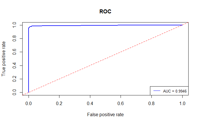
# 計算 ROC / AUC
roc = performance(prediction, "tpr", "fpr")
auc = performance(prediction, "auc")
auc = auc@y.values[[1]]
# 繪製 ROC
plot(roc, main = "ROC", col = "blue", lwd = 2)
abline(a = 0, b = 1, lty = 2, col = "red")
legend("bottomright", legend = paste("AUC =", round(auc, 4)),
col = "blue", lty = 1, cex = 0.8)
# test performance
predictions = predict(rf, newdata = new_test)
confusionMatrix(new_test$Category, predictions)

# ROC/AUC
predicted_prob = predict(rf, newdata = new_test, type = "prob")
prediction = prediction(predicted_prob[, 2], new_test$Category)

# 計算 ROC / AUC
roc = performance(prediction, "tpr", "fpr")
auc = performance(prediction, "auc")
auc = auc@y.values[[1]]

# 繪製 ROC
plot(roc, main = "ROC", col = "blue", lwd = 2)
abline(a = 0, b = 1, lty = 2, col = "red")
legend("bottomright", legend = paste("AUC =", round(auc, 4)),
       col = "blue", lty = 1, cex = 0.8)
Multinomial Naive Bayes
nb = multinomial_naive_bayes(x = new_train %>% dplyr::select(-c("Category", "Message")),
                             y = new_train$Category)
nb
# train performance
train_nb_trans = new_train %>%
  dplyr::select(-c("Category", "Message")) %>%
  as.matrix()
predictions = predict(nb, newdata = train_nb_trans)
confusionMatrix(new_train$Category, predictions)

# ROC/AUC
predicted_prob = predict(nb, newdata = train_nb_trans, type = "prob")
prediction = prediction(predicted_prob[, 2], new_train$Category)

# 計算 ROC / AUC
roc = performance(prediction, "tpr", "fpr")
auc = performance(prediction, "auc")
auc = auc@y.values[[1]]

# 繪製 ROC
plot(roc, main = "ROC", col = "blue", lwd = 2)
abline(a = 0, b = 1, lty = 2, col = "red")
legend("bottomright", legend = paste("AUC =", round(auc, 4)),
       col = "blue", lty = 1, cex = 0.8)
test_nb_trans = new_test %>%
  dplyr::select(-c("Category", "Message")) %>%
  as.matrix()

# test performance
predictions = predict(nb, newdata = test_nb_trans)
confusionMatrix(new_test$Category, predictions)

# ROC/AUC
predicted_prob = predict(nb, newdata = test_nb_trans, type = "prob")
prediction = prediction(predicted_prob[, 2], new_test$Category)

# 計算 ROC / AUC
roc = performance(prediction, "tpr", "fpr")
auc = performance(prediction, "auc")
auc = auc@y.values[[1]]

# 繪製 ROC
plot(roc, main = "ROC", col = "blue", lwd = 2)
abline(a = 0, b = 1, lty = 2, col = "red")
legend("bottomright", legend = paste("AUC =", round(auc, 4)),
       col = "blue", lty = 1, cex = 0.8)