Google PageRank
簡介
簡易範例
鄉村與都市的人口遷移問題,給定鄉村初始占總人口$x^{(0)}$的比例,都市則是$y^{(0)}$。鄉村有$p$的遷出率,都市有$q$的遷出率,則第$t$年的人口狀態可以表達為

若不考慮人口出生或死人,直覺上會覺得「無論起始值如何給定,只要時間夠長,最終一定會到收斂到平衡狀態。」即平衡狀態的存在性
與收斂性
現在將問題擴大成有$N$座城市,初始的各城市人口占比為$\bold{x}^{(0)} = (x_1^{(0)}, x_2^{(0)}, \cdots, x_N^{(0)})^T$,並用一個$N \times N$轉移矩陣 (stochastic matrix) $M$表達遷移狀態,用$M_{ij}$表達從城市$i$至城市$j$的機率。則我們有
$$ \bold{x}^{(t)} = M \bold{x}^{(t - 1)} = M^t \bold{x}^{(0)} $$設$\bold x^*$為穩定狀態,則存在性問題即討論$M$的 Eigenvector 是否存在,收斂性問題與起始點無關
$$ \bold x^* = M \bold x^* \quad \text{and} \quad \lim_{t \to \infty} \bold x^{(t)} = \bold x^* $$那最終我們可以把問題想像成
每個都市都是一個頁面,人口比例就是人們點進去這個網站的機率。
Google Pagerank
PageRank簡稱PR,是Google對搜尋結果排名的其中一個演算法。其假設為
重要的頁面會被更多其他頁面參照。
可應用於「圖論的有向性地圖權重」問題,藉由機率分布體現「某人在某個頁面的機率」。用$PR(A)$表示「某人停在$A$頁面的機率,亦表示為$A$頁面在集合內的權重」。若$PR (A) = 0.3$,則表示有0.3的機率出現在$A$頁面。而所有的頁面PR值合為1。
簡化模型
假設
- 頁面不允許自我參照;
- 頁面至少參照一個頁面;
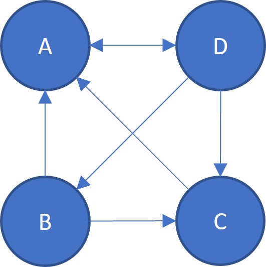
若參照情況如下

B頁面參照A與C頁面,即B給與A與C各$1/2$票。同理,也能看出D給與A、B與C各$1/3$票。故A獲得B的$1/2$票、C的1票、與D的$1/3$票。
$$ PR (A) = \frac{PR(B)}{2} + \frac{PR(C)}{1} + \frac{PR(D)}{3} $$同理
$$ PR (B) = \frac{PR (D)}{1} $$若有$N$個頁面$p_1, p_2, \cdots, p_N$,設$M (p_i)$為有參照$p_i$頁面的集合,$L (p_j)$ 為$p_j$頁面所參照的頁面數量,則任意頁面$p_i$可以寫為
$$ PR (p_i) = \sum_{p_j \in M (p_i)} \frac{PR (p_j)}{L (p_j)} $$解非唯一
在簡化模型中,會出現PR值得解非唯一的情況,考慮以下參照狀態
$$ M = \left( \begin{array}{cccc} 0 & 1 & 0 & 0 \\ 1 & 0 & 0 & 0 \\ 0 & 0 & 0 & 1 \\ 0 & 0 & 1 & 0 \\ \end{array} \right) $$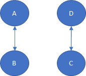
則顯然的
$$ \begin{align*} \left( \begin{array}{c} 0.25 \\ 0.25 \\ 0.25 \\ 0.25 \end{array} \right), \left( \begin{array}{c} 0.5 \\ 0.5 \\ 0 \\ 0 \end{array} \right), \left( \begin{array}{c} 0 \\ 0 \\ 0.5 \\ 0.5 \end{array} \right) \end{align*} $$都能成為解,事實上
$$ \begin{align*} \bold x = \left( \begin{array}{c} 0.5 \\ 0.5 \\ 0 \\ 0 \end{array} \right) t_1 + \left( \begin{array}{c} 0 \\ 0 \\ 0.5 \\ 0.5 \end{array} \right) t_2 \end{align*} $$對任意 $t_1 + t_2 = 1$ 都能成為解。問題出在 $\text{nullity} (M) \geq 1$,即 Eigenspace 太大使得 $\bold x$ 的解非唯一。
完整模型
上述我們做了2項假設,其中的第2假設「頁面至少參照一個頁面」,若某頁面不參照其他任何頁面,則會導致該頁面的PR值像個黑洞一樣只進不出。為防止這個情況,做出以下設定「若某頁面不參照其他頁面,則視為參照其他所有頁面。」
給定一個$d \in (0, 1)$,改變計算PR值的方式為
$$ PR (p_i) = \frac{1 - d}{N} + d \sum_{p_j \in M (p_i)} \frac{PR (p_j)}{L (p_j)} $$這邊的$d$為阻尼係數(damping factor)視為隨機瀏覽者(random surfer)根據推送到下一個頁面的機率,而$1 - d$就視為隨機到任一個網站的機率。一般預設$d = 0.85$,由一般上網者使用瀏覽器書籤功能的頻率的平均值估算得到。
原始論文版本
特別注意,PR值為機率值,我們假設
$$ \sum_{i = 1}^{N} PR (p_i) = 1 $$而在原始的版本中
$$ PR (p_i) = (1 - d) + d \sum_{p_j \in M (p_i)} \frac{PR (p_j)}{L (p_j)} $$會導致
$$ \sum_{i = 1}^{N} PR (p_i) = N \ne 1 $$因此我們不採用原始版本
矩陣形式
設定一個鄰接函數(adjacency function),由於我們假設網站不能自我參照,故任意頁面$p_i \not \to p_i$
$$ l (p_i, p_j) = \left\lbrace \begin{array}{lll} 1 / L (p_j) & \text{if} & p_j \to p_i \\ 0 & \text{if} & p_j \not \to p_i \end{array}\right. $$使得
$$ PR (p_i) = \frac{1 - d}{N} + d \cdot l (p_i, p_j) \cdot PR (p_j) $$因此用矩陣形式可以如下表達,設定$\bold x$ 為PR值組成的向量
$$ \bold x = \left( \begin{array}{c} PR (p_1) \\ PR (p_2) \\ \vdots \\ PR (p_N) \\ \end{array} \right) $$$M$是鄰接函數組成的矩陣$M_{ij} = l (p_i, p_j)$,
$$ M = \left( \begin{array}{cccc} l (p_1, p_1) & l (p_1, p_2) & \cdots & l (p_1, p_N) \\ l (p_2, p_1) & l (p_2, p_2) & \cdots & l (p_2, p_N) \\ \vdots & \vdots & & \vdots \\ l (p_N, p_1) & l (p_N, p_2) & \cdots & l (p_N, p_N) \\ \end{array} \right) $$使得$R$能以簡潔的形式表達
$$ \bold x = \frac{1 - d}{N} \textbf{1}_N + d M \bold x $$其中的$\textbf{1}_N = (1 \ 1 \ \cdots \ 1)^T \in \mathbb R^N$。
由於$\sum_{i = 1}^{n} \bold x_i = 1$,定義一個$N \times N$矩陣$E_{ij} = 1 / N$,則
$$ E\bold x = \frac{1}{N} 1_N $$故矩陣形式的$\bold x$ 可以改寫成
定義$\hat M = (1 - d) E + d M$,其中$E_{ij} = 1 / N$且$M_{ij} = l (p_i, p_j)$,則上述公式改寫
$$ \bold x = \hat M \bold x $$唯一性與收斂性
參考至 The Second Eigenvalue of the Google Matrix
計算
Power Method
起始值 $\bold x^{(0)}$ 將PR平均分配給 $N$ 個頁面,設 $\bold x^{(t)}$ 為的第 $t$ 次迭代PR值,接著重複迭代去逼近穩定狀態
$$ \begin{align*} \bold x^{(0)} & = \frac{1}{N} \textbf{1}_N \\ \bold x^{(t + 1)} & = \hat M x^{(t)} \end{align*} $$給定網站數量$N = 10$,首先隨機生成網站的參照況狀。若R[i][j]是1表示$p_i \to p_j$;反之若是0則表示$p_i \not \to p_j$。
N = 10 # Number of pages

import random
import numpy as np

R = np.zeros((N, N), dtype=int) # Reference state of pages
for i in range(N):
    for j in range(N):
        R[i][j] = 1 if random.random() < 0.3 else 0
    R[i][i] = 0
print(R)
隨機給出
[[0 0 1 0 1 0 0 0 1 0]
 [1 0 0 1 0 0 0 0 0 0]
 [1 0 0 0 0 0 1 0 0 1]
 [0 0 1 0 1 1 0 0 0 1]
 [0 1 1 0 0 0 0 1 1 0]
 [1 0 0 0 0 0 1 0 0 1]
 [0 0 1 0 0 1 0 0 0 0]
 [1 0 0 0 1 0 0 0 0 0]
 [0 0 0 1 0 1 0 0 0 1]
 [0 0 0 0 1 0 1 0 1 0]]
根據$L (p_i)$的定義為$p_i$頁面參照的總數,故$L (p_i)$等於R的列和,用L矩陣儲存$L (p_1)$、$L (p_2)$、$\cdots$、$L (p_N)$。給定$d = 0.85$並依此生成出$\hat M$
d = 0.85
N = R.shape[1] # Number of pages
L = np.array([sum(R[i]) for i in range(N)]) # Adjacency function
M = np.zeros((N, N))
for i in range(N):
    if L[i] != 0:
        for j in range(N):
            M[j][i] = R[i][j] / L[i]
    else:
        for j in range(N):
            M[j][i] = 1 / N
M_hat = d * M + (1 - d) / N
print(M_hat)
計算出$\hat M$
[[0.015      0.44       0.29833333 0.015      0.015      0.29833333
  0.015      0.44       0.015      0.015     ]
 [0.015      0.015      0.015      0.015      0.2275     0.015
  0.015      0.015      0.015      0.015     ]
 [0.29833333 0.015      0.015      0.2275     0.2275     0.015
  0.44       0.015      0.015      0.015     ]
 [0.015      0.44       0.015      0.015      0.015      0.015
  0.015      0.015      0.29833333 0.015     ]
 [0.29833333 0.015      0.015      0.2275     0.015      0.015
  0.015      0.44       0.015      0.29833333]
 [0.015      0.015      0.015      0.2275     0.015      0.015
  0.44       0.015      0.29833333 0.015     ]
 [0.015      0.015      0.29833333 0.015      0.015      0.29833333
  0.015      0.015      0.015      0.29833333]
 [0.015      0.015      0.015      0.015      0.2275     0.015
  0.015      0.015      0.015      0.015     ]
 [0.29833333 0.015      0.015      0.015      0.2275     0.015
  0.015      0.015      0.015      0.29833333]
 [0.015      0.015      0.29833333 0.2275     0.015      0.29833333
  0.015      0.015      0.29833333 0.015     ]]
給定最大迭代次數T = 100,並用record_x記錄每次x迭代的結果。
T = 100
x = np.ones(N) / N
record_x = [x]

for t in range(T):
    x = M_hat @ x
    record_x.append(x)

print(record_x[-1])
計算$\bold x^{(100)}$是
[0.12047504 0.03982829 0.14011    0.0634499  0.11683903 0.11266998
 0.1239153  0.03982829 0.1112572  0.13162697]
完整個PR函式為
N = 10 # Number of pages

import random
import numpy as np

R = np.zeros((N, N), dtype=int) # Reference state of pages
for i in range(N):
    for j in range(N):
        R[i][j] = 1 if random.random() < 0.3 else 0
    R[i][i] = 0

def PR(R: np.ndarray, T = 32, d = 0.85):
    '''
    R: Reference matirx
    T: Number of iterations
    d: Camping factor
    '''
    N = R.shape[1] # Number of pages
    L = np.array([sum(R[i]) for i in range(N)]) # adjacency function
    M = np.zeros((N, N))
    for i in range(N):
        if L[i] != 0:
            for j in range(N):
                M[j][i] = R[i][j] / L[i]
        else:
            for j in range(N):
                M[j][i] = 1 / N
    M_hat = d * M + (1 - d) / N

    x = np.ones(N) / N
    for i in range(T):
        x = M_hat @ x

    return x

print(PR(R))
結果分析
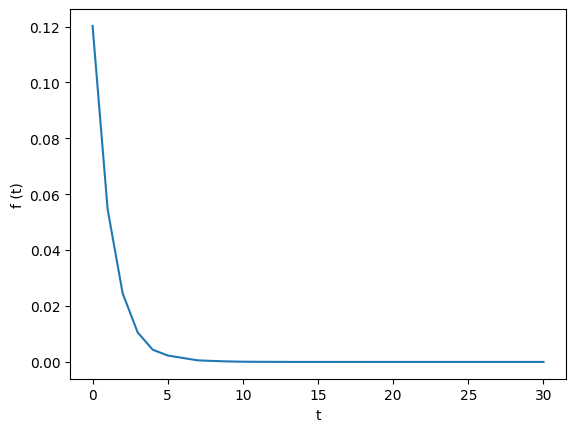
若迭代的次數足夠多,$\bold x^{(t)}$的變化量應趨近於$0$,即
$$ f (t) = \| \bold x^{(t)} - \bold x^{(t - 1)} \|_2 \to 0 $$並觀察$\bold x^{(t)}$的收斂速度
$$ g (t) = f (t - 1) / f (t) $$from numpy import linalg as LA
import matplotlib.pyplot as plt
import math
f = [LA.norm(record_x[t] - record_x[t - 1]) for t in range(1, T)]
log_f = [math.log(f[i]) for i in range(1, T - 1)]
g = [f[t - 1] / f[t] for t in range(1, T - 1)]
plt.figure(0)
plt.xlabel('t')
plt.ylabel('f (t)')
plt.plot(f)
plt.figure(1)
plt.xlabel('t')
plt.ylabel('ln f(t)')
plt.plot(log_f)
plt.figure(2)
plt.xlabel('t')
plt.ylabel('g (t)')
plt.plot(g)
發現$f (t)$隨著$t$上升而遞減
且$\ln f (t)$與$t$的關係大約呈現線性
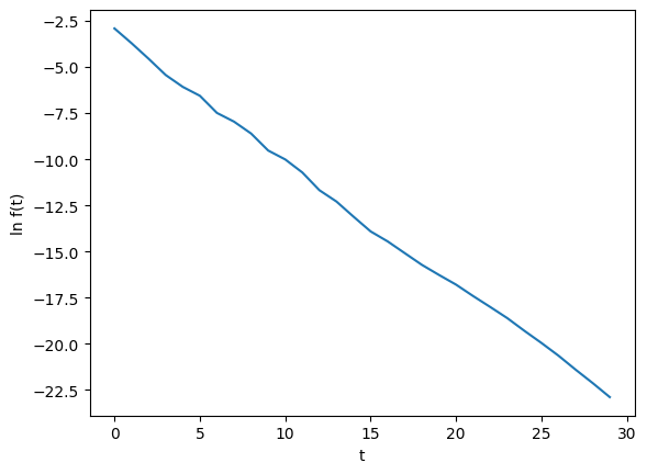
假設$\log f (t)$滿足線性關係使得,則可解出$a = - \frac{2}{3}$與$b = - \frac{5}{2}$,即
$$ f (t) \approx 10^{- \frac{2}{3} t - \frac{5}{2}} $$而$g (t)$則在2左右波動,滿足前面的假設
$$ g (t) = \frac{f (t - 1)}{f (t)} \approx e^{2/3} \approx 1.95 $$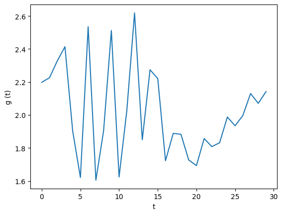
觀察多次實驗,在$N = 10、$ $d = 0.85$與「0.3的隨機參照機率」的條件下多次嘗試
- PR值的誤差逐漸縮小,即$f (t) \to 0$
- PR值得誤差量每次約少2倍,即$g (t) \approx 2$
特別注意,在最開始生成C矩陣的時候,任意頁面參照其他頁面的機率設為0.3,即
我認為收斂速度會被下列因素影響
- 頁面數量$N$,數量越多收斂越慢
- 阻尼係數$d$,不確定影響關係
- 隨機參照機率,不確定影響關係
附件
原始文獻
- BRIN, Sergey; PAGE, Lawrence. The anatomy of a large-scale hypertextual web search engine. Computer networks and ISDN systems, 1998, 30.1-7: 107-117.
Google 的資料
Google搜尋引擎的資料庫收錄超過千億網頁,檔案大小超過100,000,000 GB。
https://www.google.com/search/howsearchworks/how-search-works/organizing-information/
新算法
根據Google前員工的說法,”PageRank自2006年以來就沒有被使用過”,取而代之的新算法是